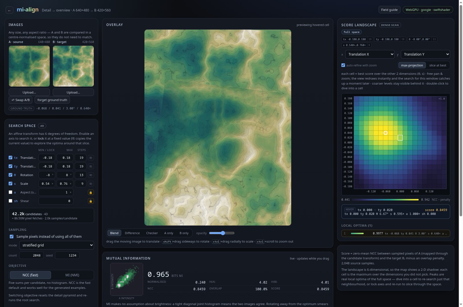
A technical note on brute-force affine alignment: canonical coordinates, NCC and mutual-information scoring, when feature matching fails, and a WebGPU compute kernel that scores a whole grid of transforms at once.
The standard approach to image alignment is to detect distinctive features, match them between the images, and estimate a homography from the resulting correspondences. That works well when the images share repeatable features and enough of them survive robust matching. It fails when the features are not shared, are repeated, or are too sparse — and then there is no correspondence set from which to estimate the geometry.
This note is about a different organisation of the problem: score a dense grid of candidate affine transforms, keep the whole score field, and study its landscape. The interesting technical questions are what to score, how to search the space, and why the computation maps well onto WebGPU.
Six numbers, one transform
Both images are mapped into a centred canonical frame, so the same parameter values describe a small detail and a large overview. For a pixel in an image of size :
The candidate transform maps canonical coordinates of the moving image A into canonical coordinates of the fixed image B:
That gives six degrees of freedom:
| Axis | Meaning |
|---|---|
tx, ty | translation in normalised image units |
θ | rotation |
s | uniform scale |
a | aspect ratio |
sh | shear |
A representative grid is candidates. Fixing an axis removes it from the product and lets the remaining axes be sampled more finely. The search space is not artificially bounded: parameter ranges can extrapolate beyond the original grid rather than clipping at the boundary.
Scoring a candidate
A candidate is scored by sampling pixels from A, mapping them through the candidate transform into B, and comparing the two intensity sequences with a zero-mean normalised cross-correlation:
NCC is invariant to brightness and contrast rescaling and lies in . The final score subtracts a penalty for samples that fall outside B:
Candidates below a minimum overlap are rejected. Without that guard, a tiny patch of B that happens to match a few samples could win by hiding most of the moving image outside the frame.
When NCC is not enough: mutual information
NCC assumes that corresponding pixels have a roughly linear intensity relationship. That is a good assumption for many photographs, but it is not universal. Two images of the same scene can come from different sensors with completely different contrast curves — or from different physical modalities altogether.
The alternative is an area-based metric. Instead of matching features, mutual information asks how much knowing the intensity in A reduces the uncertainty about the intensity in B. It is built from entropy:
The normalised form is bounded:
The joint histogram is the picture to keep in mind. When the images are aligned, a bright pixel in A tends to pair with a bright pixel in B, and the joint histogram collapses onto a diagonal. When they are misaligned, the pairs are scrambled and the histogram spreads out.
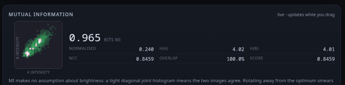
The joint histogram is estimated from paired intensities. A tight diagonal means the images agree; a diffuse distribution means they do not.
This matters most when feature detection fails. Keypoint-based registration needs the same distinctive points to be detectable and matchable in both images. That breaks down when the features are hard to match, repeated, or present in only one modality. A visible-light photograph and an X-ray or XRF element map are the classic example: they can show entirely different features, yet their intensities are still statistically dependent when the images are aligned.
This is not an argument against feature matching. For same-modality pairs, corner and edge detectors plus SIFT/ORB descriptors and RANSAC are usually the best first choice: panorama stitching, multi-view RGB, repeated scans, and even exposure or scale changes share plenty of repeatable landmarks, and a sparse set of good matches is enough to recover the geometry. Cross-modality is where the correspondence assumption itself fails: a feature that is strong in one image may be invisible in the other, descriptor matching produces false positives, and RANSAC cannot recover a transform from too few inliers. Entropy-based metrics such as MI avoid the correspondence problem by scoring the joint intensity distribution over the whole overlap; that is why they are standard in multimodal medical registration and in the MA-XRF artwork case below. They are more expensive, but they are solving a harder problem.
| Situation | Feature matching (SIFT/ORB + RANSAC) | Entropy / MI |
|---|---|---|
| Panorama stitching, multi-view RGB | Usually the best first choice: plentiful shared corners and edges | Works, but usually unnecessary and slower |
| Same modality, exposure or scale changes | Often good after contrast normalisation; repeated textures can produce false matches | Robust to monotonic intensity changes |
| RGB vs. X-ray / thermal / XRF | Fragile: landmarks not shared, false positives, too few inliers for RANSAC | Better fit: scores the whole overlap without correspondences |
| Repeated or low-texture structure | Ambiguous matches; manual tie points may be needed | Still needs signal, but avoids discrete matching failure |
Entropy-based methods are not a universal replacement. They become the better tool when the correspondence assumption is the problem, not merely when the pixels look different. NCC is cheaper, but may be less effective when the intensity relationship is not linear or the images come from different modalities.
Villafañe et al. use exactly this idea to register macro X-ray fluorescence (MA-XRF) element maps of paintings to the visible image. The modalities may share no common features, so feature-based methods are often ineffective; MI still has a signal to optimise. See Multimodal image registration and mosaicking of artworks: an approach based on mutual information, Proc. SPIE 12620, 1262004 (2023), doi:10.1117/12.2673427.
Entropy-based MI is expensive. Every candidate needs its own joint histogram, marginals and entropy sums. An NCC scorer only accumulates five running sums per candidate, while an MI scorer clears and atomically updates a histogram per candidate. NCC is cheaper, but it can be less effective when the intensity relationship is not linear or the images come from different modalities.
Brute force on the GPU
The brute-force scan is embarrassingly parallel: every candidate is independent. The host builds the cartesian product of the enabled axes, packs each candidate as a 6-float affine, and streams the matrices to the GPU in batches of 8,192.
For each candidate, one compute workgroup is dispatched. Its 128 invocations stride over the sampled source pixels, transform each one into B, bilinearly fetch B from a texture, and accumulate the sums needed for NCC and overlap. A tree reduction in workgroup shared memory combines the lane totals; invocation 0 writes the final row. The MI objective keeps the same shape but gives every candidate a private joint histogram.
WebGPU - a simpler more flexible computing model
The kernel shape is not an accident. WebGL's fragment pipeline was built for rendering, and using it for general computation means bending the graphics model into a different job. A fragment shader is tied to the pixel it is rendering: one invocation, one output location, no arbitrary scatter. A non-trivial compute job becomes a sequence of shader programs and render targets, with textures ping-ponged between passes and the pipeline organised around which pass reads and writes which texture. WebGL also has no compute stage, storage buffers, workgroup shared memory or atomics, so reductions and histograms have to be expressed as extra passes.
Floating-point data is another source of friction. In WebGL, floating-point render targets are an extension and are not universally available; the fallback is to encode each float into RGBA8 bytes, pack it in one pass and unpack it in the next. That costs precision, adds instructions to every read and write, and makes the data path harder to reason about. The companion article The Challenges of WebGL goes through these constraints in detail.
WebGPU exposes the computing model directly: compute pipelines with @workgroup_size(128), f32 storage buffers for candidate matrices and score rows, workgroup shared memory for the tree reduction, atomics for the MI histogram, and texture sampling for image B. dispatchWorkgroups(candidateCount) maps one workgroup to one candidate; @builtin(local_invocation_index) maps one lane to one strided subset of samples. There are no render passes to organise just to do arithmetic, no ping-pong textures, and no float-packing layer. The API is more verbose than a WebGL draw call, but the model is simpler for this kind of work: buffers in, dispatch, buffers out. The same device and queue can also render the visualization, so compute and graphics share one resource model.
A personal note: I finally got to test WebGPU on Linux after switching from an Nvidia GPU to an AMD one. That made this project practical to build and benchmark on the machine I actually use.
The arithmetic is straightforward:
A scan is about 122 million sample fetches. On a GPU that is one dispatch per batch; on a CPU it is a scheduling problem.
Projecting the N-D landscape
A six-dimensional score field cannot be drawn at once. The natural 2-D view is a max-projection: choose two axes and, for every cell, take the maximum over all remaining axes. An isolated peak in that shadow is a genuine local optimum of the full space. The complementary view is a slice: fix the hidden axes at the best transform and show the true 2-D cross-section.
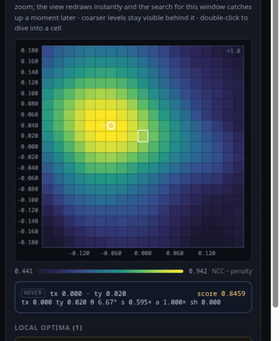
Each cell is the maximum over the hidden axes. Brighter cells score better; the rings mark local optima.
The projection can be evaluated over an arbitrary window in parameter space. Re-running the search over the visible window produces a finer level of a detail pyramid; coarser levels retain context and share a colour scale, so the refined patch remains comparable with its surroundings. Local maxima of the projected field are the candidates worth refining further, and a search over a single cell or a fixed slice reduces the dimensionality of the next pass.
Summary
Brute-force affine alignment makes the score function the centre of the design. NCC is cheap enough to scan a dense grid; entropy-based MI is more expensive but handles cross-modality pairs where feature correspondences do not exist. The computation is a grid of independent reductions, which maps directly onto WebGPU workgroups, storage buffers, shared memory and atomics. WebGL's fragment pipeline would require a chain of render passes and float packing for the same work.
The implementation used for the figures is at github.com/nikhedonia/mi-align.
Related Articles
Hamilton: A Phase-Space Playground
Type a Hamiltonian or Lagrangian, integrate it in the browser, and watch an entire phase space evolve. A WebGL2 playground with RK4, symbolic derivatives and 21 built-in systems.
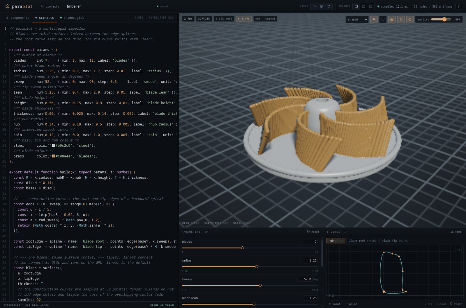
Paraplot: From Scene Code to a Draw Call
How a browser CAD toy compiles a JavaScript scene into a scene graph, one fragment shader and a uniform pool — and where late-bound edits and each kind of variable enter the pipeline.
The Challenges of WebGL
WebGL lets you run shaders in the browser — and that's genuinely magical. But using it for arbitrary GPU computation quickly reveals a thicket of constraints that OpenCL and WebGPU were designed to escape.