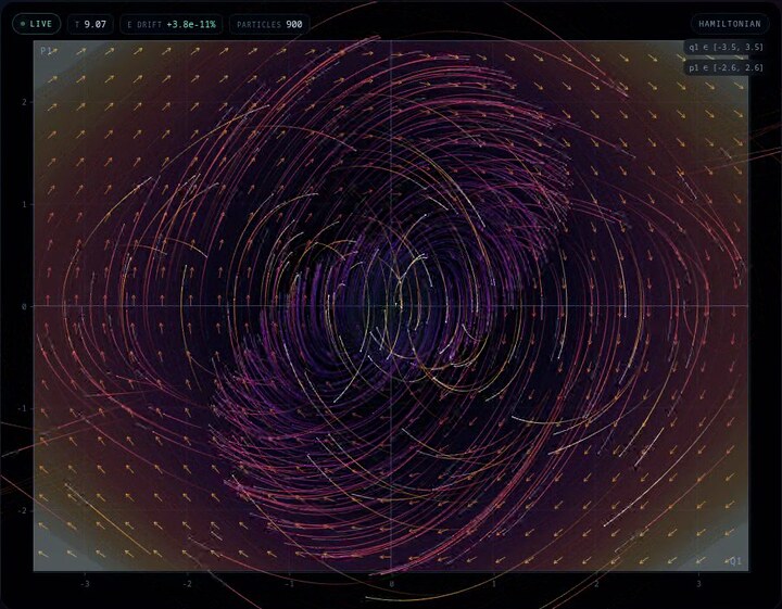
Type a Hamiltonian or Lagrangian, integrate it in the browser, and watch an entire phase space evolve. A WebGL2 playground with RK4, symbolic derivatives and 21 built-in systems.
Most simulations show one trajectory. Phase space shows the whole story at once: every possible state, organized by energy, with the flow drawn as a field.
Hamilton is a browser playground for that picture. You can type a Hamiltonian or a Lagrangian , pick one of 21 examples, and watch a cloud of initial conditions trace out the dynamics.
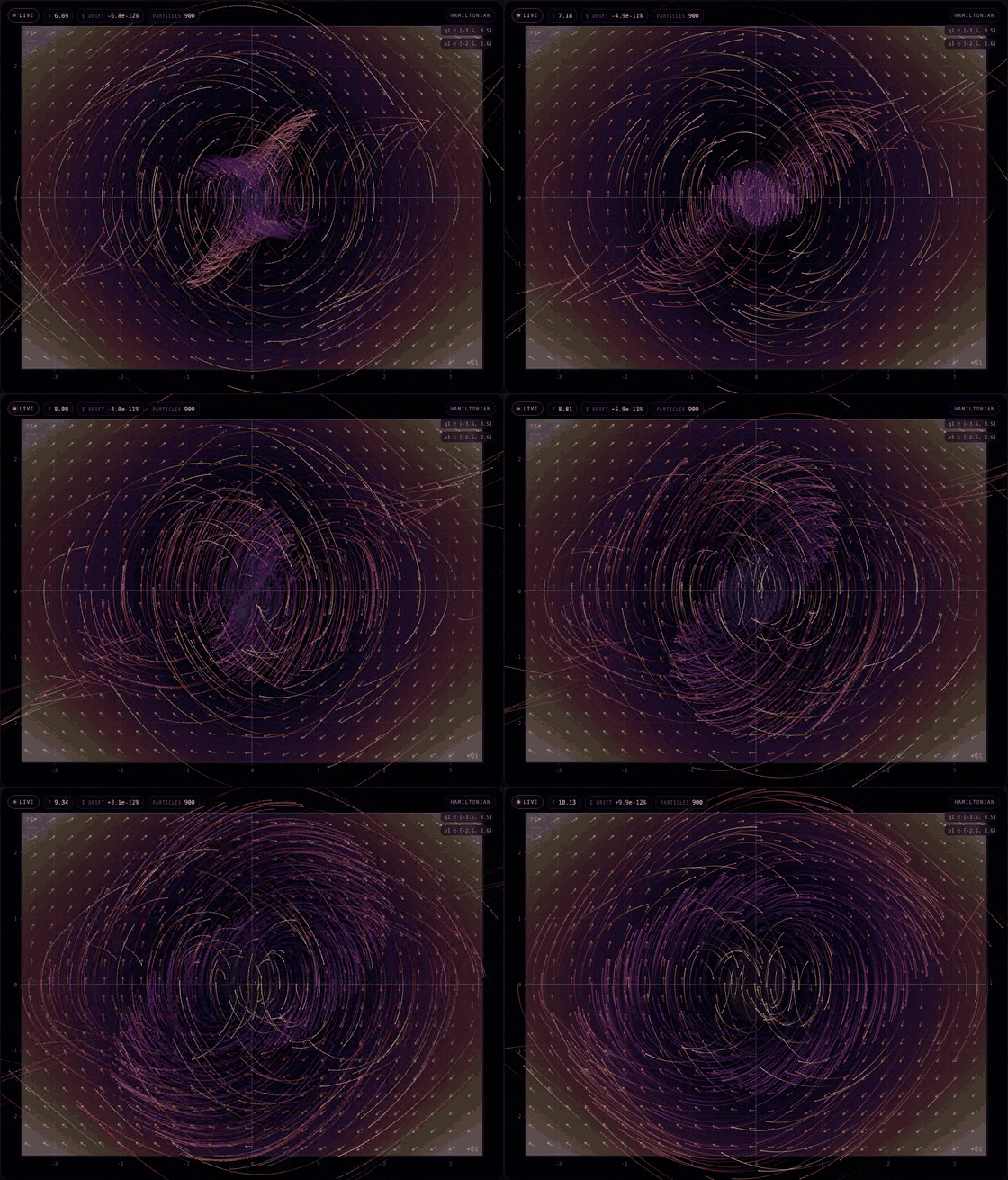
Coupled pendulums. The background is an energy slice; the trails are recent trajectories; the colour encodes each orbit's initial energy.
What it does
- Solves 1D and 2D conservative systems.
- Takes a Hamiltonian or a Lagrangian as an expression, with editable parameters and constants.
- Differentiates the expression symbolically, then compiles it to plain JavaScript for the integrator.
- Integrates with fixed-step Runge–Kutta 4 inside a Web Worker.
- Draws the energy landscape, the flow arrows, live particle trails and a static phase portrait in WebGL2.
- Includes a built-in field guide explaining the physics, the visual layers and the expression syntax.
For a Hamiltonian, the flow is first order in positions and canonical momenta:
For a Lagrangian, the app solves the Euler–Lagrange equations as a small mass-matrix system:
The Lagrangian examples are integrated in , while the energy colour still comes from the Legendre transform .
Why phase space is worth looking at
A single orbit tells you what one initial condition does. Phase space shows the structure around it: stable centres, saddle points, separatrices, periodic islands and chaotic seas. The pendulum's separatrix, a double well's figure-eight, the precessing orbits of a softened Kepler potential and the onset of chaos in the double pendulum all become geometric objects instead of lists of numbers.
For two degrees of freedom the full state is four-dimensional. The playground shows a two-dimensional projection; the background holds the hidden coordinates at zero, while the trajectories themselves still move through the full space. Change the axes and you see another shadow of the same system.
Open the playground: nikhedonia.net/hamilton
Drag to pan, scroll to zoom, and press Space to pause. The Guide button explains the rest.
Under the hood
The interesting part is the loop between mathematics and pixels: expressions are parsed into a tree, differentiated symbolically and turned into JavaScript closures; a worker steps the state and computes the energy field; the main thread only uploads transferable buffers and issues WebGL draw calls. A GPU ring buffer keeps the fading trails cheap.
The source and the full set of examples are in the Hamilton repository, and the short project write-up is under Projects. If you want to start somewhere, open the Pendulum, compare its Hamiltonian and Lagrangian versions, then try the Double pendulum and watch two nearby initial conditions disagree.
Related Articles
The Challenges of WebGL
WebGL lets you run shaders in the browser — and that's genuinely magical. But using it for arbitrary GPU computation quickly reveals a thicket of constraints that OpenCL and WebGPU were designed to escape.
Conformal Maps: When Complex Functions Preserve Angles
A conformal map preserves angles: near every point it behaves like a rotation followed by a uniform scaling. Explore them in a playground that warps grids and images — written with complex numbers, 2D vectors, and dual numbers.
Automatic Differentiation
A deep-dive into automatic differentiation: symbolic vs. numerical vs. AD, AST transformation, dual numbers, tapes, hybrid methods, and a generic C++ implementation that computes gradients and solves optimisation problems.